Simulated butterfly dataset

To illustrate the power of IntegrAO, we include an example of applying IntegrAO to simulated butterfly datasets originally coming from butterfly images. We use two different common encoding methods (Fisher Vector (FV) and Vector of Linearly Aggregated Descriptors (VLAD) with dense SIFT) to generate two different vectorizations of each image. These two encoding methods describe the content of the images differently and therefore capture different information about the images.

The first dataset has 1032 samples and the second has 1132 samples. There are 832 common samples from the 2 datasets, which means 200 samples are unique for dataset1 and 300 samples are unique for dataset2. The IntegrAO will perform integration for all the samples and product a final graph of union 1332 samples

Import packages and IntegrAO code

import numpy as np
import pandas as pd
import snf
from sklearn.cluster import spectral_clustering
from sklearn.metrics import v_measure_score
import matplotlib.pyplot as plt

import sys
import os
import argparse
import torch

import umap

# Add the parent directory of "integrao" to the Python path
module_path = os.path.abspath(os.path.join('../'))
if module_path not in sys.path:
    sys.path.append(module_path)

from integrao.dataset import GraphDataset
from integrao.main import dist2
from integrao.integrater import integrao_integrater

Set hyperparameters

torch.cuda.is_available()

True

# Hyperparameters
neighbor_size = 20
embedding_dims = 64
fusing_iteration = 20
normalization_factor = 1.0
alighment_epochs = 1000
beta = 1.0
mu = 0.5
dataset_name = 'butterfly'

Read data

# read the data
testdata_dir = os.path.join(module_path, "data/butterfly/")
w1_ = os.path.join(testdata_dir, "w1.csv")
w2_ = os.path.join(testdata_dir, "w2.csv")
w1 = pd.read_csv(w1_, index_col=0)
w2 = pd.read_csv(w2_, index_col=0)

label = ["label"]
w1_label = w1[label]
w2_label = w2[label]
wcom_label = w1_label.filter(regex="^common_", axis=0)
w1.drop(label, axis=1, inplace=True)
w2.drop(label, axis=1, inplace=True)
wall_label = pd.concat([w1_label, w2_label], axis=0)
wall_label = wall_label[~wall_label.index.duplicated(keep="first")]

print("W1 shape: ", w1.shape)
print("W2 shape: ", w2.shape)

W1 shape:  (1032, 500)
W2 shape:  (1132, 500)

wall_label

	label
common_0	1
common_1	1
common_2	1
common_3	1
common_4	1
...	...
x2_1127	10
x2_1128	10
x2_1129	10
x2_1130	10
x2_1131	10

1332 rows × 1 columns

UMAP plot for w1 and w2 before integration

import matplotlib.pyplot as plt
import umap.umap_ as umap


# Create UMAP reducer
reducer = umap.UMAP(n_neighbors=30, min_dist=1.0, spread=1.0)
embedding_w1 = reducer.fit_transform(w1.values)

# UMAP projection for w2
reducer = umap.UMAP(n_neighbors=30, min_dist=1.0, spread=1.0)
embedding_w2 = reducer.fit_transform(w2.values)

# Create a figure with two subplots
plt.figure(figsize=(20, 8))

# First subplot for w1
plt.subplot(1, 2, 1)
plt.scatter(
    embedding_w1[:, 0],
    embedding_w1[:, 1],
    c=w1_label.values.tolist(),
    s=6,
    cmap="Spectral",
    alpha=1.0,
)
plt.gca().set_xticks([])
plt.gca().set_yticks([])
plt.title("UMAP projection of w1 before integration", fontsize=18)
plt.colorbar()

# Second subplot for w2
plt.subplot(1, 2, 2)
plt.scatter(
    embedding_w2[:, 0],
    embedding_w2[:, 1],
    c=w2_label.values.tolist(),
    s=6,
    cmap="Spectral",
    alpha=1.0,
)
plt.gca().set_xticks([])
plt.gca().set_yticks([])
plt.title("UMAP projection of w2 before integration", fontsize=18)
plt.colorbar()

# Show the plot
plt.show()

Let’s check the clustering perforamance before integration

Dist1 = dist2(w1.values, w1.values)
Dist2 = dist2(w2.values, w2.values)

S1 = snf.compute.affinity_matrix(Dist1, K=neighbor_size, mu=mu)
S2 = snf.compute.affinity_matrix(Dist2, K=neighbor_size, mu=mu)

labels_s1 = spectral_clustering(S1, n_clusters=10)
score1 = v_measure_score(w1_label["label"].tolist(), labels_s1)
print("Before diffusion for full 1032 p1 NMI score: ", score1)

labels_s2 = spectral_clustering(S2, n_clusters=10)
score2 = v_measure_score(w2_label["label"].tolist(), labels_s2)
print("Before diffusion for full 1132 p2 NMI score:", score2)

Before diffusion for full 1032 p1 NMI score:  0.5778190029790612
Before diffusion for full 1132 p2 NMI score: 0.59024832833319

IntegrAO integration

# Initialize integrater
integrater = integrao_integrater(
    [w1, w2],
    dataset_name,
    neighbor_size=neighbor_size,
    embedding_dims=embedding_dims,
    fusing_iteration=fusing_iteration,
    normalization_factor=normalization_factor,
    alighment_epochs=alighment_epochs,
    beta=beta,
    mu=mu,
)

# IntegrAO
fused_networks = integrater.network_diffusion()
embeds_final, S_final, model = integrater.unsupervised_alignment()

labels = spectral_clustering(S_final, n_clusters=10)

score_all = v_measure_score(wall_label.sort_index()["label"].tolist(), labels)
print("IntegrAO for clustering intersecting 1332 samples NMI score: ", score_all)

Start indexing input expression matrices!
Common sample between view0 and view1: 832
Neighbor size: 20
Start applying diffusion!
Diffusion ends! Times: 15.384316444396973s
Starting unsupervised exmbedding extraction!
Dataset 0: (1032, 500)
Dataset 1: (1132, 500)
epoch 0: loss 25.31028175354004, align_loss:0.224211
epoch 100: loss 18.538162231445312, align_loss:0.052776
epoch 200: loss 1.8779222965240479, align_loss:0.019808
epoch 300: loss 1.8769832849502563, align_loss:0.019133
epoch 400: loss 1.875892162322998, align_loss:0.018408
epoch 500: loss 1.8746706247329712, align_loss:0.017648
epoch 600: loss 1.873340129852295, align_loss:0.016874
epoch 700: loss 1.871917486190796, align_loss:0.016102
epoch 800: loss 1.8703994750976562, align_loss:0.015341
epoch 900: loss 1.8687971830368042, align_loss:0.014590
Manifold alignment ends! Times: 60.17931294441223s
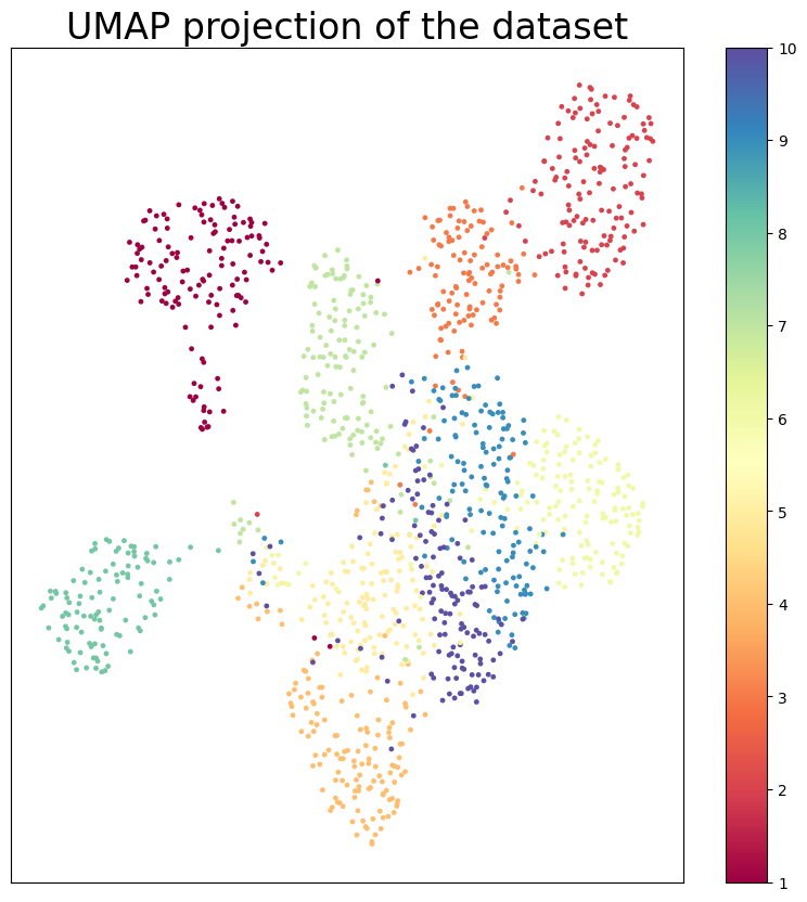
IntegrAO for clustering intersecting 1332 samples NMI score:  0.7704099811263375

UMAP plot of the integrated embeddings

import umap

# umap visualization of embeddings with hue as labels
reducer = umap.UMAP(n_neighbors=30, min_dist=1.0, spread=1.0)
embedding = reducer.fit_transform(embeds_final.values)
plt.figure(figsize=(10, 10))
plt.scatter(
    embedding[:, 0],
    embedding[:, 1],
    c=wall_label.sort_index()["label"].tolist(),
    s=6,
    cmap="Spectral",
    alpha=1.0,
)
plt.setp(plt.gca(), xticks=[], yticks=[])
plt.title("UMAP projection of the dataset", fontsize=24)
plt.colorbar()
plt.show()